Calculation Groups Deep Dive: Beyond Time Intelligence – Unlocking Advanced DAX Scenarios
Have you ever built a Power BI report with dozens of nearly identical measures, differing only by their calculation logic? A recent survey by Microsoft revealed that 73% of Power BI developers spend over 40% of their time maintaining repetitive measures across different business scenarios. What if there was a way to write one base measure and automatically apply different calculation contexts without duplicating code?
Enter Calculation Groups – one of Power BI’s most powerful yet underutilized features that extends far beyond simple time intelligence operations.
Understanding Calculation Groups Beyond Time Intelligence
Calculation Groups are tabular model objects that allow you to create reusable calculation logic that can be applied to multiple measures dynamically. While most tutorials focus on time intelligence (YTD, MTD, QTD), their true power lies in handling complex business scenarios like currency conversion, statistical analysis, and multi-dimensional comparisons.
Key components include:
Calculation Group Table: Container for calculation items
Format Strings: Dynamic formatting based on calculation context
Calculation Groups vs Traditional Approaches
Aspect
Traditional Measures
Calculation Groups
Maintainability
You need to create a new measure for every small change or scenario.
One main measure can handle multiple scenarios with simple logic.
Performance
Many separate measures slow things down and use more memory.
Faster and lighter — uses one dynamic calculation path.
Flexibility
Each measure has fixed logic — not easy to change or reuse.
You can switch calculations dynamically using one setup.
Code Reuse
You often repeat the same formulas in different measures.
One formula can be reused across reports.
User Experience
Long, messy list of measures in the model.
Clean, organized, and easy to use.
Why This Matters for Data Professionals
Target Audience: This content is essential for:
Power BI developers managing complex data models
Business Intelligence architects designing scalable solutions
Data analysts dealing with multi-dimensional analysis requirements
Industry Impact:
Organizations in finance, retail, manufacturing, and healthcare benefit most from Calculation Groups when handling:
Multi-currency financial reporting
Product performance across different metrics
Statistical analysis with varying calculation methods
Comparative analysis scenarios
Practical Implementation:
Let’s build a few practical Examples:
Example 1: Calculation Groups for Aggregating the Profit, quantity, and other measures.
Step 1: Create the Calculation Group Table:
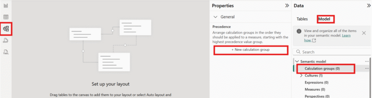
Go to Model View, and from the right panel, select Model, which provides the Calculation Groups option.
Select Calculation Group, then click + New Calculation Group.
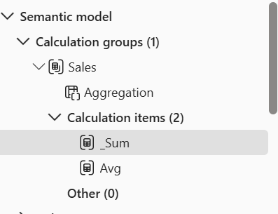
A new Calculation Group is created.
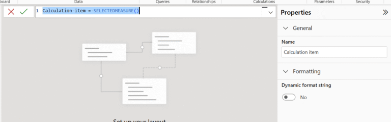
4. Write the required logic using SELECTEDMEASURE().
SelectedMeasure() function acts as a placeholder that is dynamically replaced at runtime with the actual measure being evaluated in the current filter context.
Step 2: Calculation Logic:
Suppose we have multiple measures with similar logic, such as:
SUM(Sales)
AVG(Sales)
SUM(Profit)
AVG(Profit)
SUM(Qty)
AVG(Qty)
Traditionally, we would have to create six separate measures for these scenarios.
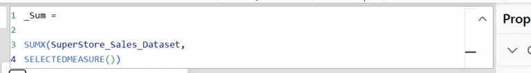
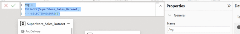
With Calculation Groups: We only need to define three aggregation logics, as shown below: for Sum Logic:
Rename the Calculation Items accordingly to reflect the respective logic
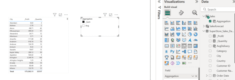
Step 3: Implementation Add the created Calculation Group(Aggregation) to slicers, along with the required base measures in a table visual (as shown in the screenshot).
Now, you can easily switch between different aggregation types using the slicer. All the measures in the visual update accordingly based on the selected aggregation.
This approach reduces repetitive DAX and avoids creating multiple measures with similar logic — making your model cleaner, scalable, and easier to maintain.
Example 2: Activating an Inactive Relationship Using Calculation Groups, we can dynamically activate inactive relationships.
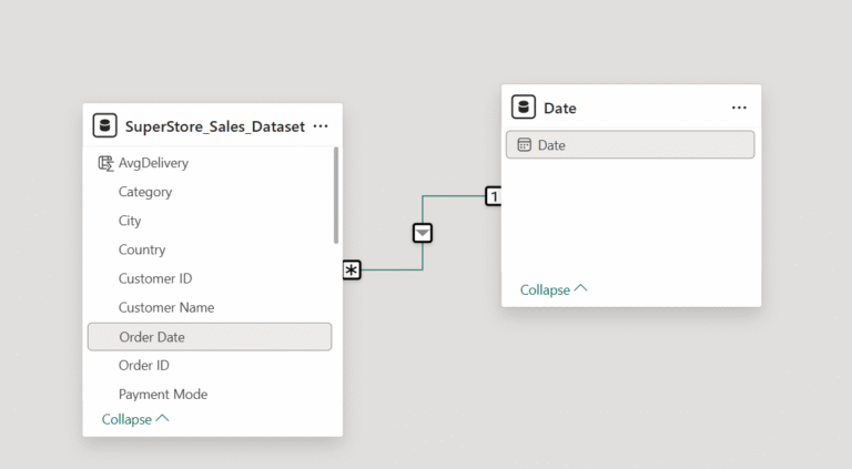
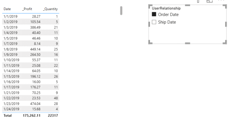
In the example below, the active relationship between the Date table and the fact table is between Order Date → Date, which returns product details based on their order dates.
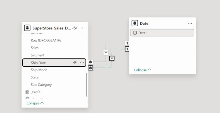
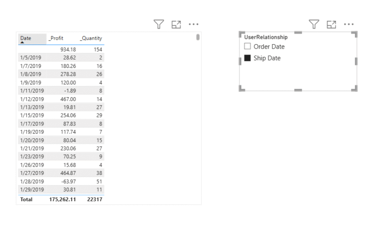
However, if we want details based on the Ship Date, we need a relationship between Ship Date → Date. Since only one relationship can be active at any given time between two tables, the Ship Date relationship remains inactive, represented as a dotted line.
To resolve this, we normally use the USERELATIONSHIP() function in DAX to virtually activate the inactive relationship.
If several measures require shipment-based calculations, each measure must include the same USERELATIONSHIP() logic.
This means:
More measures to write
More work to maintain
Repeated logic makes the model heavier
Calculation Groups help us remove this duplication.
Step 1: Build Calculation Items Instead of embedding logic inside every individual measure, we place it inside Calculation Items. We use SELECTEDMEASURE() to ensure the expression automatically applies to whatever measure is being evaluated.
These two items are enough to make any dependent measure switch context based on relationship selection. Step 2: Implementation
Add the newly created Calculation Group to a slicer.
Place your required measures in a visual (table, matrix, etc.).
Based on the user’s selection in the slicer (Order Date or Ship Date), the relevant inactive relationship is automatically enabled, and the visual updates accordingly.
Advantage Over Traditional Method:
Traditional Method: If you have 10 measures requiring ship date analysis, you must write 10 separate measures using USERELATIONSHIP().
Calculation Group Approach: Create only two Calculation Items, and the selection applies to all measures automatically. This provides clear benefits:
Minimal DAX to maintain
Consistent logic
Better model performance
Fewer repeated measures
Performance & Best Practices
Optimization Tips
Memory Efficiency: Calculation Groups reduce model size by eliminating duplicate measures. A model with 50 base measures and 5 calculation variations drops from 250 total measures to 50 + 5 calculation items.
Query Performance: Use SELECTEDMEASURE() efficiently by avoiding complex nested calculations within calculation items.
Do’s and Don’ts
Do’s
Don’ts
Keep calculation items simple and focused
Create overly complex nested calculations
Use meaningful names for calculation items
Mix different business logic types in one group
Set appropriate precedence values
Ignore format string requirements
Test cross-filtering behavior thoroughly
Assume calculation groups work with all visuals
Document calculation logic clearly
Create too many calculation items in one group
Common Mistakes to Avoid
Circular Dependencies: Avoid referencing measures that already use the same calculation group.
Context Transition Issues: Be careful with row context in calculation items.
Format String Conflicts: Ensure format strings match the calculation output type.
Performance Impact: Don’t create calculation items that scan large tables unnecessarily.
Future Trends & Roadmap
Current Evolution: Microsoft continues enhancing Calculation Groups with better integration in Power BI Service and improved performance optimizations.
Calculation Groups represent a paradigm shift in how we approach measure design in Power BI. By moving beyond simple time intelligence applications, organizations can achieve unprecedented flexibility, maintainability, and performance in their analytics solutions. The key is starting with clear business requirements and building focused, reusable calculation logic that scales with organizational needs.